Practical Guide to Building an Accurate Customer Lifetime Value Prediction

Have you ever wondered how valuable a customer really is to your business—not just today but over the entire course of their relationship with you? That’s where customer Lifetime Value comes in. It’s a way to predict the total revenue a customer will bring to your business throughout their entire journey with your brand.

Now, imagine you’re deciding how much to invest in acquiring new customers or retaining existing ones. Wouldn’t it be invaluable to know which customers are likely to stick around and contribute the most to your bottom line? CLV prediction allows you to do just that. Understanding the financial value of each customer allows you to:

• Make smarter, more targeted marketing decisions.
• Optimize resource allocation.
• Strengthen loyalty programs to keep your best customers coming back.

By the end of this guide, you’ll know how to use CLV in your own business. Whether you’re just getting started or refining your strategy, there’s something here for everyone. Let’s dive in and turn your customer data into a tool for growth!

Understanding Customer Lifetime Value

Customer Lifetime Value (CLV) represents the projected net profit from a customer over their entire relationship with a company. It factors in revenue, acquisition, and service costs. A reliable customer lifetime value prediction empowers companies to:

• Tailor marketing efforts to high-value customers.
• Make data-driven decisions for customer retention.
• Adjust budgets based on expected long-term profitability.

Guide to Predict Customer Lifetime Value (CLV)

Now that we have discussed the meaning of Customer Lifetime Value (CLV), let’s go over how to predict CLV step by step. It covers everything from data preparation to model building, validation, and deployment. By the end of this guide, you’ll be equipped with the knowledge and tools to calculate and implement CLV predictions effectively.

The code used in this guide has been re-implemented from this GitHub repo.

Step 1: Identifying and Preparing Data Sources

Begin by gathering and structuring high-quality data. Learn the essential data types (e.g., transactional, demographic, and behavioral data) and how to preprocess them for accurate modeling.

Data Requirement

To accurately predict Customer Lifetime Value (CLV), gather the following types of data:

• Transactional Data: Purchase frequency, transaction amounts, and timestamps.
• Demographic Data: Basic customer details like age, location, and acquisition source.
• Behavioural Data: Engagement metrics such as browsing history or product interaction.
• Historical CLV (optional): Use this as a benchmark to validate predictions.

Data Preparation

Once your data is ready, follow these steps to clean and prepare it for prediction.

Acquire Data

In this guide, we will work with the online retail dataset from the UCI Machine Learning repository. This transactional data set contains all transactions occurring between 01/12/2010 and 09/12/2011 for a UK-based and registered non-store online retail.

import pandas as pd
import numpy as np

data = pd.read_csv("/content/Online Retail.csv", encoding="unicode_escape", parse_dates=['InvoiceDate'])

Note: If you’re a ClicData user, simply use our native data connectors to your eCommerce platform, database and API connectors and store it in your data warehouse in ClicData.   

Feature Selection

For our prediction, we don’t need all the features in the dataset. We need only the CustomerID, InvoiceDate, Quantity, and TotalSales.

So, we keep only these features and drop all the others.

features = ['CustomerID', 'InvoiceNo', 'InvoiceDate', 'Quantity', 'UnitPrice']
data_clv = data[features]
data_clv.head()

Feature Engineering

Derive TotalSales per transaction feature from UnitPrice and Quantity.

data_clv['TotalSales'] = data_clv['Quantity'].multiply(data_clv['UnitPrice'])
data_clv.head()

This is what our data looks like after performing these initial preparation steps:

Step 2: Data Quality Checks

Ensure your data is clean and reliable. This includes handling missing values, removing duplicates, and summarizing key statistics to verify data readiness.

Handle Missing Data

In our Customer Lifetime Value prediction calculation, we are interested only in the total value a customer can generate for the business over a lifetime. 

• We will simply drop negative values in TotalSales and work with only positive values. 
• Also, drop the null values in the CustomerID variable.

data_clv = data_clv[data_clv['TotalSales'] > 0]
data_clv = data_clv[pd.notnull(data_clv['CustomerID'])]

Quick Dataset Summary

Here is the summary of the data after performing the cleaning steps:

maxdate = data_clv['InvoiceDate'].dt.date.max()
mindate = data_clv['InvoiceDate'].dt.date.min()
unique_cust = data_clv['CustomerID'].nunique()
tot_quantity = data_clv['Quantity'].sum()
tot_sales = data_clv['TotalSales'].sum()

print(f"Time Range: {mindate} to {maxdate}")
print(f"Unique Customers: {unique_cust}")
print(f"Total Quantity Sold: {tot_quantity}")
print(f"Total Sales: {tot_sales}")

Output:

Time Range: 2010-12-01 to 2011-12-09
Unique Customers: 4338
Total Quantity Sold: 5167812
Total Sales: 8911407.904

Note: You can easily clean and standardize your data using our built-in ETL module.

See how it works:

Step 3: Selecting a Modeling Approach for Prediction

Explore different modeling techniques, from simple heuristic calculations to advanced machine learning models. Understand when to use rule-based, probabilistic, or machine-learning approaches based on your dataset and prediction goals.

Types of Customer Lifetime Value Prediction Models

1. Heuristic Models

These are rule-based and simple to implement but often too simplistic. They work for businesses with limited data.

Example: Calculate customer lifetime value as 

Customer Value = Average Purchase Value x Average Number of Purchases
Customer Lifetime Value = Customer Value x Average Customer Lifespan

2. Probabilistic Models

Use distribution-based models (e.g., Gamma-Gamma or BG/NBD) to predict the probability of future purchases. Best for steady transaction data with a clear purchase pattern.

Example: The BG/NBD model predicts the probability of future transactions for each customer over a period of time, given their purchase history. To include the monetary aspect, the Gamma-Gamma model estimates the monetary value per customer based on the transaction probability.

3. Machine Learning Models

These models, especially tree-based models like Random Forest or Gradient Boosting, handle complex relationships and non-linear patterns. They are useful for a large dataset with diverse features (e.g., demographics, behavioral data).

Choosing the Right Model

• Start with Heuristic Models if your data is limited or transaction behavior is highly regular.
• Move to Probabilistic Models if you have transaction frequency data and want a relatively simple but robust model.
• Use Machine Learning Models if you can access a rich, diverse dataset and want to explore complex, non-linear relationships.

Step 4: Building the CLV Prediction Model

Why Use the BG/NBD and Gamma-Gamma Models?

The BG/NBD model predicts future transactions for each customer, while the Gamma-Gamma model estimates the monetary value of those transactions. Combined, these models calculate Customer Lifetime Value.

Feature Engineering

We will use a Python package called lifetimes for feature engineering. This package is primarily built to aid customers in their lifetime value calculations. It has all the major models and utility functions that are needed for CLV calculations.

! pip install lifetimes

First, we need to create a summary table from the transaction data. The summary table is an RFM (Recency, Frequency, and Monetary value) table, an aggregation of customer transaction data.

We can achieve this using the summary_data_from_transaction_data function from the lifetimes package. This function aggregates transaction-level data into customer-level data, calculating key metrics such as frequency, recency, TTT (the time frame for analysis), and monetary value for each customer.

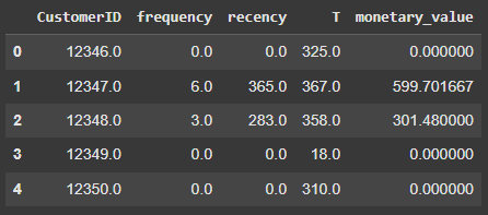
• frequency – the number of repeat purchases (more than 1 purchase)
• recency – the time between the first and the last transaction
• T – the time between the first purchase and the end of the transaction period
• monetary_value – it is the mean of a given customer sales value

import lifetimes

# Create summary data from transaction data
summary = lifetimes.utils.summary_data_from_transaction_data(
    data_clv, 'CustomerID', 'InvoiceDate', 'TotalSales')
summary = summary.reset_index()
summary.head()

Output:

For CustomerID 12347, we can observe that in 365 days (recency=365), the customer has made 6 purchases (frequency=6). The T value of 367 indicates the time we have observed the customer from their first purchase. The monetary value shows the average amount spent per transaction is 599.7. These aggregated features will provide insights for predicting customers’ future behavior.

Train the BG/NBD Model

The BG/NBD model tries to predict each customer’s future transactions.

from lifetimes import BetaGeoFitter
bgf = BetaGeoFitter()
bgf.fit(summary['frequency'], summary['recency'], summary['T'])

# Predict transactions for the next 30 days
t = 30
summary['pred_num_txn'] = bgf.conditional_expected_number_of_purchases_up_to_time(
    t, summary['frequency'], summary['recency'], summary['T'])
summary.head()

Output:

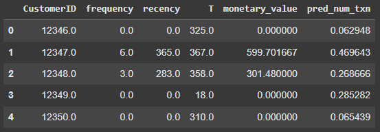
model.conditional_expected_number_of_purchases_up_to_time(): Calculate the expected number of repeat purchases up to time t for a randomly chosen individual from the population (or the whole population), given their purchase history (frequency, recency, T).

In the code above, the t=30 represents the period, i.e., the next 30 days, and we are predicting how many purchases each customer is likely to make during the next 30 days based on their previous history.

Train the Gamma-Gamma Model

Now that we predicted the expected future transactions, we need to predict the future monetary value of each transaction.

The BG/NBD model can only predict a customer’s future transactions and churn rate (the rate at which customers stop doing business with a company over a period of time). To add the monetary aspect to the problem, we have to model the monetary value using the Gamma-Gamma Model.

For this analysis, we focus only on customers who have made repeat purchases with the business (i.e., those with frequency > 0). Customers with a frequency of 0 are considered one-time purchasers and are treated as “already churned.” This approach ensures the monetary value predictions are relevant and meaningful for active repeat customers.

from lifetimes import GammaGammaFitter

summary = summary[summary['frequency'] > 0]
ggf = GammaGammaFitter()
ggf.fit(return_customers['frequency'], return_customers['monetary_value'])

# Calculate the expected average profit per transaction
summary['exp_avg_sales'] = ggf.conditional_expected_average_profit(
    summary['frequency'], summary['monetary_value'])
summary.head()

Output:

model.conditional_expected_average_profit(): This method computes the conditional expectation of the average profit per transaction for a group of one or more customers.

Calculating Customer Lifetime Value

Now, we will combine the predictions from the BG/NBD and Gamma-Gamma models to calculate CLV.

model.customer_lifetime_value(): This method computes the average lifetime value of a group of one or more customers. This method takes in the BG/NBD model and the prediction horizon as a parameter to calculate the CLV.

summary['predicted_clv'] = ggf.customer_lifetime_value(
    bgf, summary['frequency'], summary['recency'], summary['T'], summary['monetary_value'],
    time=1,  # Prediction horizon in months
    freq='D',  # Frequency of transactions
    discount_rate=0.01  # Discount rate for future cash flow
)
summary.head()

You can also calculate the CLV manually from the predicted number of future transactions (pred_num_txn) and expected average sales per transaction (exp_avg_sales).

summary['manual_predicted_clv'] = summary['pred_num_txn'] * summary['exp_avg_sales']

This is what the data looks like after predictions:

Model Validation

Validate your predictions using error metrics such as Mean Absolute Error (MAE) and Root Mean Squared Error (RMSE). This ensures your model is accurate and reliable for business decision-making.

Error Metrics Explained

• Mean Absolute Error (MAE): Represents the average magnitude of prediction errors, offering a straightforward measure of accuracy.
• Root Mean Squared Error (RMSE): Captures the standard deviation of prediction errors, highlighting how concentrated the errors are around the mean.

from sklearn.metrics import mean_absolute_error, root_mean_squared_error

mae = mean_absolute_error(summary['predicted_clv'], summary['manual_predicted_clv'])
rmse = root_mean_squared_error(summary['predicted_clv'], summary['manual_predicted_clv'])

print(f"Mean Absolute Error (MAE): {mae}")
print(f"Root Mean Squared Error (RMSE): {rmse}")

Output:

Mean Absolute Error (MAE) : 2.388740115190495Root Mean Square Error (RMSE) : 8.100815583510194

These values represent the model’s average prediction error (MAE) and the standard deviation of these errors (RMSE), helping you understand the model’s predictive accuracy.

Step 5: Implementing and Deploying the Model in Production

Deployment brings your model into action. Decide whether predictions must be real-time or batch-based, and choose the right deployment platform.

Deployment and Automation

1. Batch Predictions: Schedule predictions weekly or monthly, depending on business needs.
2. Real-Time Predictions: Use APIs to serve predictions instantly, ideal for high-traffic applications.

import joblib

# Save the models
joblib.dump(bgf, '/content/bgf_model.pkl')
joblib.dump(ggf, '/content/ggf_model.pkl')


# Load the models
loaded_bgf_model = joblib.load('/content/bgf_model.pkl')
loaded_ggf_model = joblib.load('/content/ggf_model.pkl')


# Perform Predictions
loaded_bgf_model.conditional_expected_number_of_purchases_up_to_time(
    t, summary['frequency'], summary['recency'], summary['T'])
loaded_ggf_model.conditional_expected_average_profit(summary['frequency'], summary['monetary_value'])

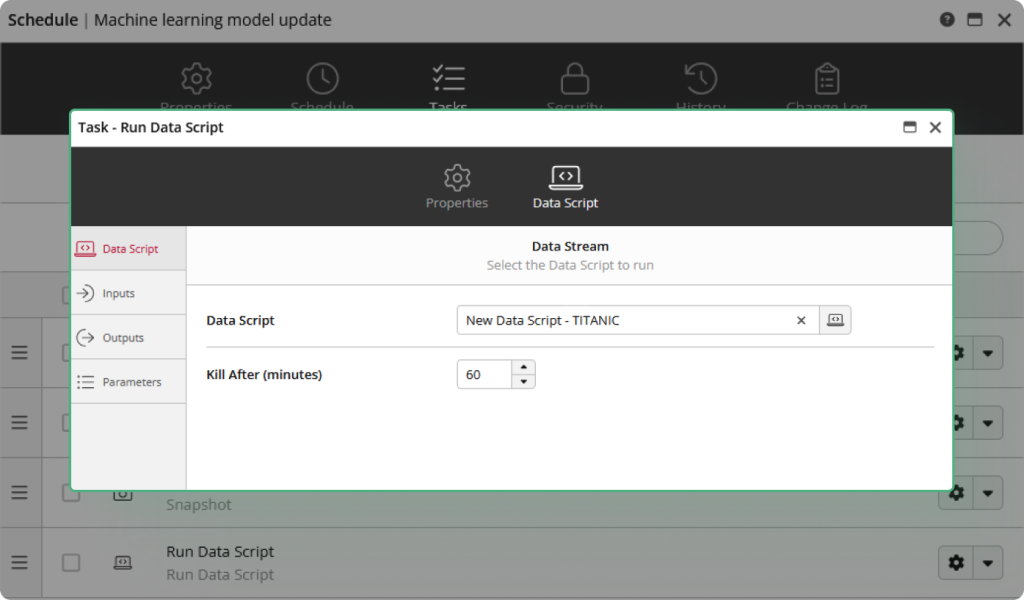
ClicData provides a user-friendly interface for scheduling the execution of your script and feeding your dashboards with the latest customer lifetime value prediction outputs. 

Step 6: Monitoring and Retraining

Automate retraining based on performance. Set up alerts if metrics (e.g., MAE, RMSE) degrade. Again, you can set up these custom automatic alerts in ClicData.

Common Pitfalls and Solutions

Customer lifetime value prediction significantly impacts business strategies, but several pitfalls can undermine it. This section will identify and solve those challenges to keep our results reliable and actionable.

Using Insufficient or Low-Quality Data

CLV models are unlikely to produce accurate predictions without comprehensive and high-quality data. Missing values, inconsistent formats, and irrelevant features can distort the model’s output.

For example, A CLV model trained on incomplete transactional data with missing purchase dates or order values may overestimate or underestimate CLV, leading to misinformed marketing strategies.

Regularly inspect your dataset for missing or incorrect values to ensure data quality. Use methods such as df.isnull(), df.sum(), or df.describe() to identify anomalies and inconsistencies effectively. If you encounter missing values in key features like total cost, consider filling with median or mean values, or drop rows selectively if there are few enough to remove without impact.

data_clv = data_clv[data_clv['TotalSales'] > 0]

Always ensure data completeness and consistency before modeling.

Failing to Update the Model Regularly

Customer behaviors change, especially with seasonal patterns, economic shifts, or changes in product offerings. A CLV model built on outdated data may quickly become inaccurate.

For example, a model trained on data from a high-spending holiday season may predict an inflated CLV for the next quarter if it is not updated with new data.

Set up a pipeline to automatically retrain your model on recent data. This can be done monthly, quarterly, or on a schedule that suits your business needs.

Track metrics like Mean Absolute Error (MAE) over time. An increase in error rates may indicate that the model needs retraining.

def monitor_drift(y_true, y_pred):
    mae = mean_absolute_error(y_true, y_pred)
    if mae > some_threshold:
        print("Model drift detected! Consider retraining the model.")

A model is only as good as the data it’s trained on. Regular updates maintain relevance.

Focusing Solely on Revenue and Ignoring Churn

CLV is not just about predicting revenue; it’s also about understanding retention. Many CLV models overlook churn predictions, which can lead to an overestimation of customer value.

For example, a CLV model may forecast high future value for customers who are likely to churn in the next quarter, skewing profitability expectations.

Include churn probability as a feature in your CLV model, especially in subscription or recurring-revenue businesses.

Use models like Kaplan-Meier or Cox Proportional-Hazards to estimate the probability that a customer will remain active over time.

Accounting for churn refines your CLV estimates and makes them more actionable.

Overfitting with Complex Models

Overfitting happens when a model captures noise rather than patterns, leading to high accuracy on training data but poor performance on new data. Complex machine learning models (like random forests or XGBoost) are especially prone to overfitting if not controlled.

Example: A tree-based model with too many splits may perfectly predict training data but fail on unseen data due to memorizing details rather than learning general patterns.

Use L1/L2 regularization to penalize overly complex models. Limit maximum tree depth or set minimum sample split thresholds for tree-based models.

from xgboost import XGBRegressor
model = XGBRegressor(max_depth=5, learning_rate=0.1, reg_lambda=1.0) 

# Train model on selected features
X = df[['frequency', 'recency', 'monetary_value', 'T']]
y = df['clv']

model.fit(X, y)

Then, use k-fold cross-validation to verify the model’s performance on different data splits. This will help you detect and correct overfitting.

Simpler models with regularization often perform better for CLV prediction.

Using Customer Lifetime Value Predictions for Business Impact

With customer lifetime value predictions in place, let’s look at how they can drive business value.

Applications of Customer Lifetime Value Predictions

1. Customer Segmentation: Target high-value customers with retention and upsell offers.
2. Marketing Optimization: Personalize campaigns and allocate budgets based on customer lifetime value predictions.
3. Product Improvements: Identify customer needs by segment and tailor services accordingly.

Measuring Impact

Use indicators such as customer retention rates, ROI on marketing spend, and customer acquisition cost (CAC) to measure the impact of your customer lifetime value model.

Predict Your Customer Lifetime Value With ClicData

As we have already covered, building an accurate customer lifetime value prediction model involves aligning data, model selection, and deployment with business goals.

Start with simpler models, experiment with advanced techniques as data permits, and always keep the business needs in mind!

If you want to start building your customer lifetime value prediction, check out our cloud-based Python scripting tool integrated into a full-fledged data management and analytics platform. Connect your data, store it in a built-in data warehouse, cleanse and standardize it, and develop your CLV model in one platform.

Test it or book a 1:1 session with our data experts to see it live!