SQL may not be the newest tool in your stack, but it’s still what you reach for when it counts. Whether you’re debugging a broken KPI, slicing some metrics for an executive request, or tracing a slow query that is blocking your dashboard, SQL is truly at the center of every data operation you perform.
However, we all know that writing SQL that’s not just correct, but clean, scalable, and fast, is an entirely different skill than just being confident with it.
This guide will take you through 20 ways to write better SQL. To kick things off, in the first half, we will focus on fundamental habits like formatting, filtering, and clean aliases that allow you to build faster and easier-to-understand queries.
Then, in the second half, we’ll level up with advanced techniques: window functions for rankings and trends, pivots for reshaping data, smart use of joins and CTEs, and battle-tested strategies for dealing with messy data at scale.
Let’s dive in!
Data Setup: Customers and Orders
Before getting started with the interesting part, we need to introduce the data we’ll be using throughout the whole guide. To keep this guide practical and consistent, we’ll use two simple yet realistic tables throughout the examples:
- Customers
This table contains key customer information such as region, sign-up date, lifetime revenue, and who referred them (if any).
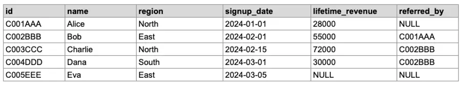
We’ll use a dummy customers table throughout the examples
- Orders
This table tracks all customer purchases, with dates, categories, and order amounts spread across 2024.
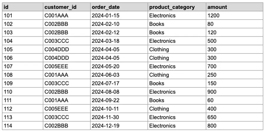
We’ll use a dummy orders table throughout the examples
Feel free to recreate them in your local environment to follow along and test queries hands-on.
Part 1: Core SQL Habits
Before diving into complex queries or advanced techniques, it’s essential to get the basics right. Writing better SQL isn’t just about mastering functions; it’s about developing smart habits that make your code cleaner, safer, and easier to maintain.
Basic SQL Tips
To be better at writing SQL, there’s no need to craft more complex queries. It is a matter of writing smarter ones. Small improvements in your SQL habits can make your code safer, more understandable, and more optimal.
Let’s start with five basic steps in this direction.
#1 Add Comments to Your Queries
Don’t overlook the value of a helpful comment. Whether you are describing a business rule or drawing attention to a challenging transformation, comments make your SQL code more informative, easier to debug, and easier to collaborate on.
Just like any other code or technical documentation out there, your SQL queries should always be clarified with comments along the code, so we can:
- Help others (and future you!) understand the logic behind your code.
- Make it easier for teammates to jump into your queries.
- Highlight key logic, edge cases, or known quirks.
There are three ways to comment in SQL.
-- Single-line comment
SELECT id FROM customers;

SELECT id FROM customers -- Inline comment

/*
Multiline comment
spanning several lines
*/
SELECT id FROM customers;#2 Avoid SELECT * in Production Queries
While SELECT * is a convenient statement when testing fast and getting to know tables, it comes with a high cost in production: slower queries, unnecessary data transfer, and fragile code.
So when crafting queries to be used in production, always try to specify the columns and avoid the * false friend. It will help you to:
- Reduce data volume, especially over remote or bandwidth-limited connections.
- Make your query easier to follow and debug.
- Future-proofs your code if table schemas change.
So, instead of getting all columns at once, always define the specific columns (and order) you want to select.
-- Risky
SELECT * FROM customers;
-- Better
SELECT id, name, region FROM customers;#3 Use LIMIT During Exploration
When exploring a new dataset or writing quick, ad hoc queries, the LIMIT clause is your best ally. It restricts the number of rows returned, keeping your queries lightweight. This allows you to stay in control and prevents slowdowns or crashes caused by accidentally pulling thousands (or millions) of rows.
If you are still wondering why you should care about the number of rows returned, let’s define a hypothetical scenario. Imagine scanning an entire terabyte of data just to preview a table’s structure, all because you forgot to add LIMIT at the end.
It’s a simple habit that can save you time, resources, and potentially costly mistakes.
You can easily add it at the end of your SQL queries, just as follows.
SELECT
id,
order_date,
amount
FROM orders
LIMIT 10;#4 Format for Readability
SQL is not only meant for machines; it is meant for humans as well.
This includes you, your future you, and anyone else that you may collaborate with. This is why clean, well-formatted SQL is much easier to read, maintain, and debug. To do so, just follow these guidelines;
- For SQL keywords, use UPPERCASE (SELECT, FROM, WHERE)
- Indent nested logic and subqueries
- Break long queries into logical sections
- Align JOIN, ON, and WHERE clauses consistently
Let’s test it out with the following example.
Imagine I share with you the following (extremely short) query.
select id, name, region from customers where lifetime_revenue > 0 and signup_date >'2024-01-01'It is hard to read, right?
As it is all written in a single line of code, we cannot understand the inner structure of the query at a single glance. However, if we now consider the previous best practices, we would get something as follows.
SELECT
  id,
  name,  region
FROM
  customers
WHERE
  lifetime_revenue > 0
AND signup_date > '2024-01-01';With this example, we can easily break down the query, since it uses a consistent format that everyone is familiar with.
Pro tip: Some teams prefer placing commas at the beginning of each line. This makes it easier to catch missing commas when editing:
SELECT
  id
  ,name  ,region
FROM
  customers
WHERE
  lifetime_revenue > 0
AND signup_date > '2024-01-01';Whatever style you choose, stick to it. A SQL formatter (like SQLFormat, or your IDE’s built-in tool) can help enforce consistency.
#5: Double-Check Filters in UPDATE/DELETE
Destructive queries require extra caution. Forgetting a WHERE clause in an UPDATE or DELETE can wipe or alter an entire table in seconds. So when altering data contained in our table, always keep in mind:
- To preview with SELECT.
- To double-check WHERE clauses do what we want them to do.
- To back up before running in production.
- To test changes in a dev environment.
So always follow these two logical steps:
-- Step 1: Verify affected rows
SELECT *
FROM customers
WHERE customer_id = 'C001AAA';

-- Step 2: Run the actual change
DELETE
FROM customers
WHERE customer_id = 'C001AAA';Remember: Your WHERE clause is your safety net. Respect it.
Foundational Querying Best Practices
Once you’ve mastered the basics, it’s time to begin writing cleaner and more maintainable SQL queries. This section is aimed at helping you avoid logic errors that can often be subtle, and write queries that can grow in terms of complexity with your projects and team members.
#6 Learn the SQL Execution Order
SQL looks like it runs top to bottom, but it doesn’t.
One of the most common areas for error in SQL comes from not understanding how queries are executed under the hood. Although you write SQL starting with SELECT, generally, databases will execute queries in a different logical order:
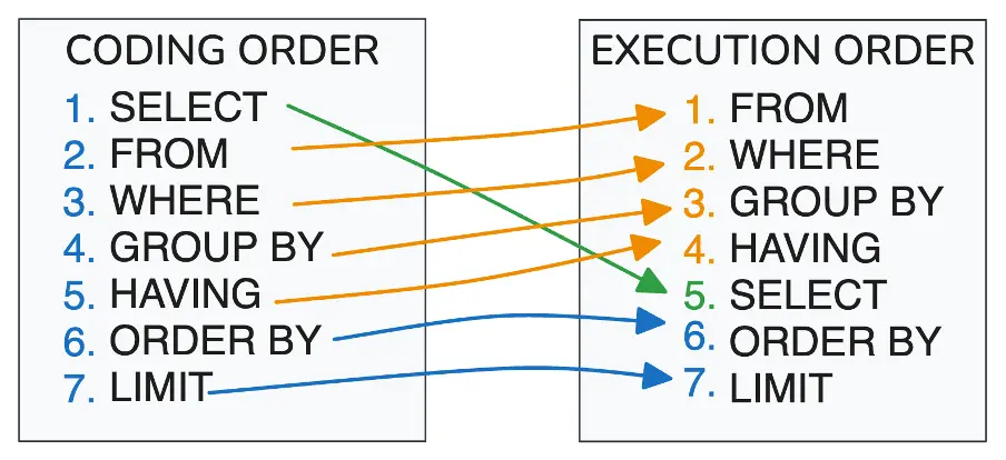
Image 1: Difference between SQL coding and execution order.
So… why is it important to understand the execution order of SQL?
- This helps you debug queries more easily.
- It prevents logic errors (like trying to filter on aggregated columns in WHERE)
- It enables performance tuning by rethinking where operations happen.
Once you understand this execution flow, you’ll write more efficient and accurate queries.
Let’s look at this example:
SELECT
  customer_id,
  COUNT(*) AS total_orders
FROM orders
WHERE amount > 100
GROUP BY customer_id
HAVING COUNT(*) > 2
ORDER BY total_orders DESC;The execution order could then be:
- FROM orders
- WHERE amount > 100
- GROUP BY customer_id
- HAVING COUNT(*) > 2
- SELECT
- ORDER BY
If you try to use HAVING before aggregation or put filtering logic after SELECT, you’ll run into errors or unexpected results.
#7 Use Descriptive Aliases
Aliases are your friend for the clarity and maintainability of your queries.
Remember, SQL queries need to be read and maintained by humans. Consequently, we should always keep in mind to make these queries more understandable and friendly.
So, let’s see what happens when I show you the following query.
SELECT
  sud,
  ltr
FROM cus c;Do you understand what kind of data I’m dealing with?
You might get ‘cus’ comes from customers, but you most likely won’t get anything else. There are no hints to help us understand what we are fetching and working with.
So instead of using cryptic abbreviations or default column names, try to assign a descriptive alias to tables and fields.
Something like the following:
SELECT
  cus.signup_date,
  cus.lifetime_revenue
FROM customers cus;In this case, the query is self-explanatory.
Pro tip: Avoid one-letter aliases in production code unless you’re writing quick one-liners or explorations. Always keep in mind the standardization terms you have in your company and stick to them.
#8 Understand WHERE vs HAVING
To summarize and filter data effectively, WHERE and HAVING are your go-to clauses. However, most people get confused when using them, even though they serve different purposes.
- WHERE filters rows before any aggregation happens.
- HAVING filters groups after aggregation is performed.
This means that while WHERE filters rows (original from our table), HAVING filters groups after an aggregation process. So let’s see how both work using simple queries as examples.
SELECT
product_category,
COUNT(*) AS order_count
FROM orders
WHERE amount > 100
GROUP BY product_category;In the first query, we use WHERE amount > 100 to filter the raw data before grouping. This ensures only rows that fulfill the defined condition are included in the aggregation.
SELECT   product_category,
COUNT(*) AS order_count
FROM orders
GROUP BY product_category
HAVING COUNT(*) > 2;In the second query, we don’t filter by category but instead group all products and then use HAVING COUNT(*) > 2 to keep only those product groups with more than 2 orders.
So always keep in mind to use WHERE when filtering individual rows and use HAVING when filtering on aggregates.
#9 Handle NULLs Intentionally
In SQL, NULL means unknown, not zero or empty. This means that if you treat nulls like any other value, you most likely will end up having problems with your code.
The most common mistake is to use the equal symbol (=) to locate null values in SQL, just like follows.
-- Always returns nothing
WHERE column = NULLThe previous command will output a null table. Instead, you can use the IS and IS NOT clauses to locate all the nulls in your table.
-- Good way to detect null values
WHERE column IS NULL
WHERE column IS NOT NULLOnce we have found all of our nulls in our table, we can just replace them using the ISNULL or COALESCE functions.
- ISNULL(expr, replacement) that replaces NULL with a default value
- COALESCE(val1, val2, …) that returns the first non-null value
SELECT
  name,
  ISNULL(title, 'Unnamed') AS clean_name
FROM customers;Always think critically about how your data handles missing values, and design queries accordingly.
#10 Use CTEs to Modularize Complex Queries
If your SQL is too long and contains multiple subqueries within, it’s time to switch to CTEs (Common Table Expressions).
CTEs let you break a big query into readable, testable, and reusable blocks, like LEGO pieces. Each CTE block represents one transformation step, helping you debug and collaborate more effectively. By leveraging CTEs in our SQL queries, we can:
- Improve readability and separation of logic.
- Simplify debugging step by step.
- Avoid repeating logic (we can reuse the same block for multiple queries).
- Enhance teamwork by modularizing complex queries.
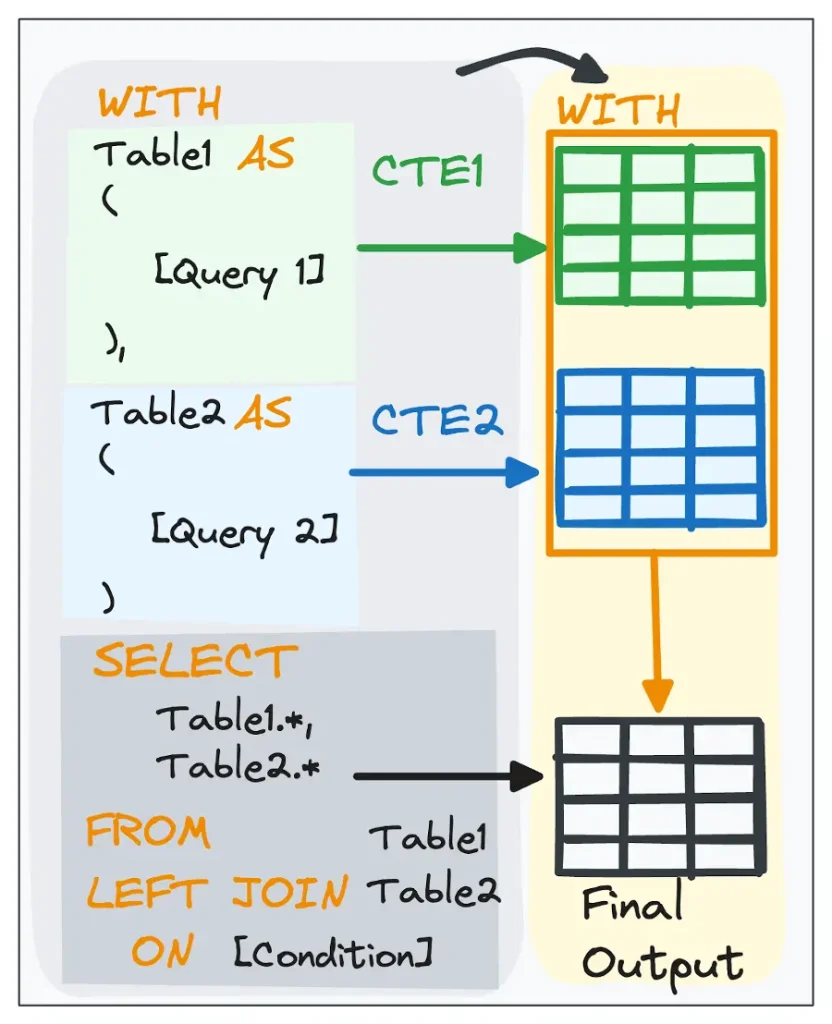
Image 2: Understanding CTEs.
To maintain CTEs clean and reusable:
- Use clear, descriptive CTE names.
- Keep each CTE focused on one task.
- Chain steps logically for clarity and maintainability.
Here’s a standard query that finds all customers who signed up in 2024 and shows their total order value.
SELECT
summary.name,
summary.total_orders,
summary.total_spent
FROM (
SELECT
c.customer_id,
c.name,
COUNT(*) AS total_orders,
SUM(o.amount) AS total_spent
FROM customers c
JOIN orders o
ON c.customer_id = o.customer_id
WHERE c.signup_date >= '2024-01-01'
GROUP BY c.customer_id, c.name
) AS summary
WHERE summary.total_orders > 2
AND summary.total_spent > 1000
ORDER BY summary.total_spent DESC;It works, but the logic is packed into one block, which makes it harder to understand, test, or reuse. Let’s modularize the same query using CTEs.
-- Step 1: Filter customers who signed up in 2024
WITH

recent_customers AS (
SELECT *
FROM customers
WHERE signup_date >= '2024-01-01'
),

-- Step 2: Join recent customers with their orders
customer_orders AS (
SELECT
rc.customer_id,
rc.name,
o.amount
FROM recent_customers rc
JOIN orders o
ON rc.customer_id = o.customer_id
),

-- Step 3: Aggregate order counts and total amount per customer
customer_order_summary AS (
SELECT
customer_id,
name,
COUNT(*) AS total_orders,
SUM(amount) AS total_spent
FROM customer_orders
GROUP BY customer_id, name
)

-- Step 4: Filter customers with > 2 orders and > 1000 spent

SELECT
name,
total_orders,
total_spent
FROM customer_order_summary
WHERE total_orders > 2
AND total_spent > 1000
ORDER BY total_spent DESC;Each part now has a name and a purpose. We can see the corresponding tabular equivalent in the following image.

Image 3: Generating each of the temporal tables for our modular query.
It may seem trivial in short queries, but in production-level SQL with 100+ lines, using CTEs can be a lifesaver for both you and your future collaborators.
Pro Tips:
- Use descriptive names (active_users, monthly_kpis, late_orders)
- Keep each block focused on one logical transformation
- Chain multiple CTEs to create a clear narrative structure
Part 2: Advanced SQL Techniques
Now that we’ve covered the foundational habits of writing cleaner and safer SQL, it’s time to level up. In Part 2, we’ll move beyond the basics and dive into powerful techniques for transforming, aggregating, and joining data at scale.
Aggregation and Transformation Tips
When you’re building KPIs, dashboards, or trend analyses, it’s not enough to pull data; you need to transform and summarize it meaningfully. This section covers the most powerful SQL ways to do so. From grouping to pivoting and handling time-based data, these tips will help you turn raw tables into actionable insights.
#11 Filter Early with WHERE
When working with large datasets, filtering early is one of the most effective ways to boost performance and reduce costs.
A common mistake is using HAVING to filter data that could have been handled more efficiently with WHERE. As we discussed in tip #8:
- WHERE filters rows before aggregation
- HAVING filters groups after aggregation
If the condition doesn’t require aggregated values, use WHERE, as it reduces the amount of data passed through the query pipeline.
-- Efficient query (using WHERE early):
SELECT
product_category,
SUM(amount) AS total_sales
FROM orders
WHERE amount > 100
GROUP BY product_category;

-- Less efficient query (filtering late with HAVING):
SELECT
product_category,
SUM(amount) AS total_sales
FROM orders
GROUP BY product_category
HAVING SUM(amount) > 100;Rule of thumb:
Apply filters at the earliest opportunity you can, whether that’s in a WHERE clause, an early CTE, or a subquery. This helps reduce memory usage, improves performance, and lowers query cost, especially in environments based in the cloud.
Want to go deeper?
Check out this guide on reading SQL execution plans to learn how query optimizers process your SQL, and how you can spot inefficiencies before they cost you.
#12 Use Window Functions for Advanced Metrics
Window functions let you calculate metrics across rows while keeping all original rows in your result, unlike aggregate functions, which collapse data.
They’re ideal for:
- Rankings (to compute the top-selling product by revenue)
- Running totals (to compute cumulative sales over time)
- Moving averages (to compute a 3-day rolling average of sales)
- Row comparisons (to compute revenue difference from the previous period)
Mastering window functions gives you a powerful new layer of analysis in SQL, enabling you to compute complex KPIs without sacrificing row-level detail. Some of the key clauses to be used are:
- OVER() defines the “window”.
- PARTITION BY splits rows into groups.
- ORDER BY sets calculation order within the window.
Let’s see some examples in real queries.
-- Rankings - Customers by Lifetime Revenue
SELECT
  name,
  lifetime_revenue,
  RANK() OVER (ORDER BY lifetime_revenue DESC) AS revenue_rank
FROM customers
WHERE lifetime_revenue IS NOT NULL;You can observe the result of the previous query in the following image.
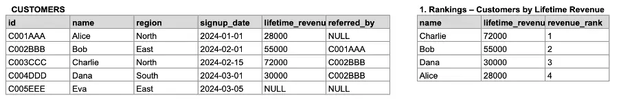
Image 4: Generating a ranking by Lifetime revenue
-- Running Totals - Total of Orders per Customer Over Time
SELECT
  customer_id,
  order_date,
  amount,
  SUM(amount) OVER (
    PARTITION BY customer_id
    ORDER BY order_date
  ) AS running_total
FROM orders;You can observe the result of the previous query in the following image.
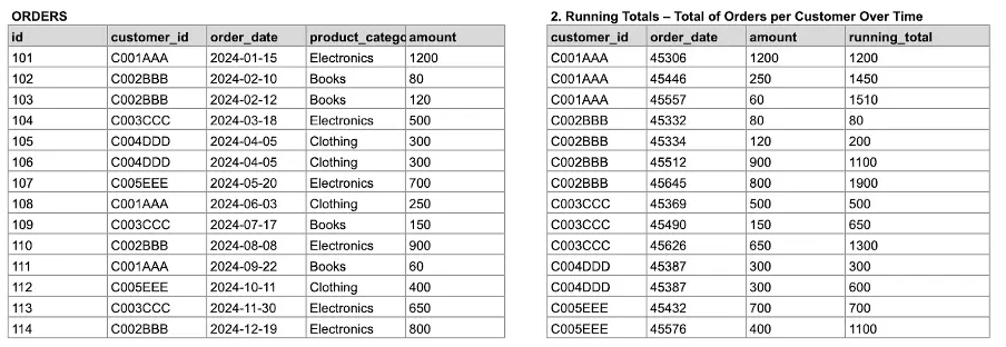
Image 5: Generating a ranking by Lifetime revenue
-- Moving Averages - 3-Order Rolling Average for Each Customer
SELECT
  customer_id,
  order_date,
  amount,
  AVG(amount) OVER (
    PARTITION BY customer_id
    ORDER BY order_date
    ROWS BETWEEN 2 PRECEDING AND CURRENT ROW
  ) AS rolling_avg
FROM orders;You can observe the result of the previous query in the following image.
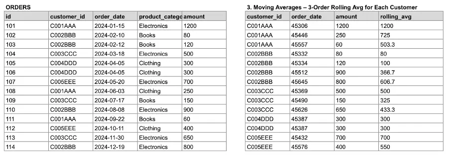
Image 6: Generating a moving average for each costumer.
-- Row Comparisons – Compare Order Amount to Previous Order
SELECT
customer_id,
order_date,
amount,
amount - LAG(amount) OVER (
    PARTITION BY customer_id
    ORDER BY order_date
  ) AS diff_from_prev_order
FROM orders;You can observe the result of the previous query in the following image.
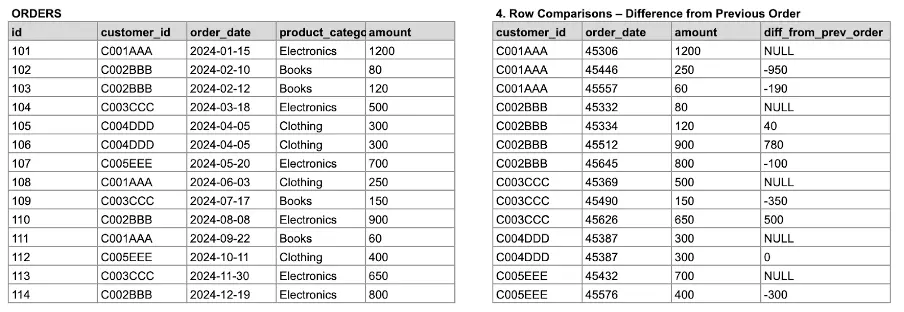
Image 7: Comparing orders with previous ones.
#13 Leverage CASE WHEN for Custom Logic
CASE WHEN operation is a built-in if-else logic in SQL. This is helpful when you want to create custom KPIs, categorize users, or segment data according to your rules.
You can use CASE WHEN in a SELECT statement, WHERE clause, ORDER BY clause, and it is even available inside of aggregates like SUM(CASE WHEN …)
SELECT
name,
lifetime_revenue,
CASE
     WHEN lifetime_revenue < 30000 THEN 'Low'
     WHEN lifetime_revenue < 60000 THEN 'Medium'
     ELSE 'High'
     END AS revenue_band
FROM customers;Pro tip: Always include an ELSE clause to handle unexpected or NULL values.
#14 Pivot and Unpivot Data When Needed
There are occasions where you will need to reshape your data: turn rows to columns or columns to rows, to fit your visualizations or reporting tools. This is where PIVOT and UNPIVOT come into play.
- PIVOT: Convert distinct values in a column to new columns (wide format), often used for dashboards or Excel-style tables.
- UNPIVOT: Convert columns to rows (long format), which is preferred by most BI and charting tools.
PIVOT: Turn Rows into Columns (Total Sales by Category per Customer)
Let’s pivot the orders table to show total spend by product_category, with one column per category:
SELECT *
FROM (
  SELECT
       customer_id,
       product_category,
       amount
       FROM orders
) AS src
PIVOT (
  SUM(amount)
  FOR product_category IN ([Electronics], [Clothing], [Books]))
AS p;This gives you one row per customer and one column per category. Much easier to visualize in a report or Excel-style table.
UNPIVOT: Turn Columns Back into Rows
Let’s say you’ve already pivoted your table and want to go back to long format:
SELECT
   customer_id,
   product_category,
   amount
FROM(
  SELECT
  customer_id,
  [Electronics],
  [Clothing],
  [Books]
  FROM customer_pivoted_orders
  ) AS p
UNPIVOT (  amount FOR product_category IN ([Electronics], [Clothing], [Books])
) AS unp;This turns the wide format back into a normalized table, perfect for trend analysis or feeding into BI tools that prefer tidy data.
You can see the difference between the pivoted and the unpivoted tables in the following example, where we have both versions from the ORDERS table.
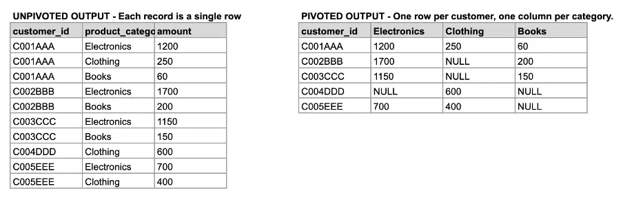
Image 8:. Pivoted and unpivoted versions of the ORDERS table.
Note on Compatibility: PIVOT and UNPIVOT are not supported in all SQL dialects. SQL Server and Oracle support them directly, but PostgreSQL, MySQL, and SQLite do not. For broader compatibility, you can achieve similar results using:
- CASE WHEN for pivoting
- UNION ALL for unpivoting
PIVOT Alternative: Using CASE WHEN
Goal: Show total amount per product category per customer, with one column per category.
SELECT
  customer_id,
  SUM(CASE WHEN product_category = 'Electronics' THEN amount ELSE 0 END) AS electronics_spent,
  SUM(CASE WHEN product_category = 'Clothing' THEN amount ELSE 0 END) AS clothing_spent,
  SUM(CASE WHEN product_category = 'Books' THEN amount ELSE 0 END) AS books_spent
FROM orders
GROUP BY customer_id;UNPIVOT Alternative: Using UNION ALL
Assume the result of the previous query is a table (or CTE) named customer_category_totals.
SELECT
  customer_id,
  'Electronics' AS product_category,
  electronics_spent AS amount
FROM customer_category_totals

UNION ALL

SELECT
  customer_id,
  'Clothing',
  clothing_spent
FROM customer_category_totals

UNION ALL

SELECT
  customer_id,
  'Books',
  books_spent
FROM customer_category_totals;#15 Use Date Functions for Time-Based Reporting
Dates are crucial in trend analysis, cohort analysis, and reporting. SQL has wonderful date functions to help you group, extract, and format date/time data.
Some common functions:
- DATE_TRUNC(): Snap timestamps to the start of a day, month, or year
- EXTRACT(): Pull components like day, week, month, or year
- DATEADD(): Shift time forward or backward
- CONVERT(): Format dates as readable strings
Here you can observe some examples:
-- Computing the monthly revenue by truncating the date to month
SELECT
  DATE_TRUNC('month', order_date) AS order_month,
  SUM(amount) AS monthly_revenue
FROM orders
GROUP BY order_month
ORDER BY order_month;You can observe in the following example the initial table (orders) and the corresponding output with the order_date truncated to the month (first day of the month).
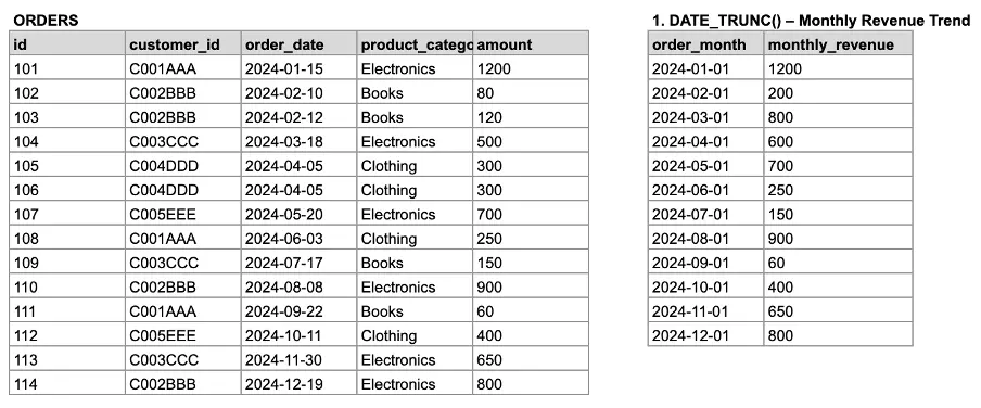
Image 9: Truncating the order date by month.
-- Extracting day of week
SELECT
 EXTRACT(DOW FROM order_date) AS weekday,
 COUNT(*) AS order_count
FROM orders
GROUP BY weekday
ORDER BY weekday;You can observe in the following example the initial table (orders) and the corresponding output with the order_date truncated to weekday.
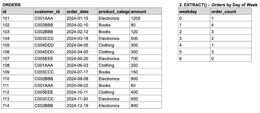
Image 10: Truncating the order date by month.
Pro tip: Use indexes wisely on date fields for optimal performance in large time-based datasets.
Joins and Subqueries
Understanding how to deal with and merge data is essential to write good SQL queries. Both JOINs and subqueries are the most essential operations from relational database querying, and one of the most used ones. This is why, if used badly, they can lead to performance bottlenecks and incorrect aggregations (and outputs).
#16 Know Your JOIN Types and When to Use Them
Joins are the real power of relational databases. Each JOIN has its purpose:
- INNER JOIN: returns the rows with matching values in both tables.
- LEFT JOIN: returns all rows from the left, plus the matching rows from the right, resulting in NULL if no match.
- RIGHT JOIN: returns all rows from the right, plus the matching rows from the left, resulting in NULL if no match.
- FULL OUTER JOIN: returns all rows from both tables, leaving NULLs for missing matches.
- CROSS JOIN: returns the Cartesian product of both tables; Use cautiously.
To make it easier to understand, you can observe the following visual.
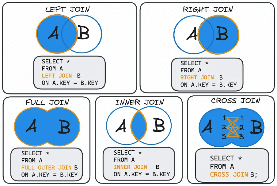
Image 11: Different types of SQL JOINs.
Pro Tip: Learn how to merge and join data in SQL visually. It is the most intuitive way to do so.
1. INNER JOIN
Returns only customers who have placed at least one order.
SELECT
  c.customer_id,
  c.name,
  o.order_id,
  o.amount
FROM customers c
INNER JOIN orders o
ON c.customer_id = o.customer_id;Use this when you only care about records that exist in both tables.
2. LEFT JOIN
Returns all customers, including those who have never placed an order.
SELECT
  c.customer_id,
  c.name,
  o.order_id,
  o.amount
FROM customers c
LEFT JOIN orders o
ON c.customer_id = o.customer_id;Helpful to find customers with no purchases (order_id will be NULL).
3. RIGHT JOIN
Returns all orders, even if they are linked to unknown customers (e.g., data mismatch or deletion).
SELECT
  c.customer_id,
  c.name,
  o.order_id,
  o.amount
FROM customers c
RIGHT JOIN orders o
ON c.customer_id = o.customer_id;Useful in data audits or incomplete datasets. Not supported in all dialects (e.g., MySQL before 8.0 lacks FULL OUTER JOIN).
4. FULL OUTER JOIN
Returns all customers and all orders, matched when possible, with NULLs where no match exists.
SELECT
  c.customer_id AS customer_id,
  c.name,
  o.order_id,
  o.amount
FROM customers c
FULL OUTER JOIN orders o
ON c.customer_id = o.customer_id;For more real-world advice on how to choose and troubleshoot JOINs, check out this practical article on mastering SQL joins.
Pro Tip:
- Use INNER JOIN for clean, matching data
- Use LEFT JOIN to detect missing matches
- Use CROSS JOIN only when you truly need every combination. We will see more about this in tip #18.
#17 Use EXISTS Instead of IN for Large Lookups
When comparing data across tables, especially large ones, EXISTS can significantly improve performance over IN. The main difference between the clauses is:
- EXISTS returns as soon as it finds the first match, making it efficient for correlated subqueries.
- IN often scans the entire list, which can be costly for large result sets.
This makes EXISTS a better choice for semi-joins when you’re just checking for the existence of related data.
-- Efficient filtering with EXISTS
SELECT
 name
FROM customers c
WHERE EXISTS (
  SELECT 1
  FROM orders o
  WHERE o.customer_id = c.customer_id
  );

-- Less efficient (especially with large datasets)
SELECT
name
FROM customers
WHERE customer_id IN (
  SELECT customer_id
  FROM orders
);Rule of Thumb:
- Use IN when checking against static or small lists
- Use EXISTS for dynamic, correlated subqueries and better performance on large datasets
#18 Be Cautious with CROSS JOIN
CROSS JOIN creates all possible row combinations between two tables. This is useful when generating scaffolding for time series, as we want a record for each product and each possible date (all products × all dates). However, it can be dangerous if used accidentally.
Let’s see a valid example of CROSS JOIN.
-- Step 1: Get distinct months from orders
WITH
distinct_months AS (
  SELECT DISTINCT
  DATE_TRUNC('month', order_date) AS month
  FROM orders
),

-- Step 2: Cross join customers with each month
customer_month_grid AS (
  SELECT
  c.customer_id,
  c.name,
  m.month
FROM customers c
CROSS JOIN distinct_months m
)

-- Optional: Left join with actual orders to find missing months
SELECT
 cm.customer_id,
 cm.name,
 cm.month,
SUM(o.amount) AS total_spent
FROM customer_month_grid cm
LEFT JOIN orders o
 ON cm.customer_id = o.customer_id
 AND DATE_TRUNC('month', o.order_date) = cm.month
GROUP BY cm.customer_id, cm.name, cm.month
ORDER BY cm.customer_id, cm.month;This helps report, gap detection, or backfilling missing values in dashboards.
Pro Tip: Avoid accidental CROSS JOINs, forgetting a JOIN condition in a FROM + JOIN clause can sometimes behave like a CROSS JOIN, resulting in huge unintended outputs.
#19 Deduplicate When Necessary
Duplicate rows can inflate metrics and slow down queries, leading to inaccurate results and inefficient processing. For example, imagine that the first two rows in the CUSTOMERS table were accidentally repeated three times each.
Deduplication means identifying and removing these duplicates, either by eliminating rows that are exact copies across all columns, or by targeting specific columns (or a combination of them) to keep only unique values.
The following image shows a visual example of this process:
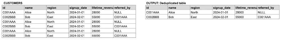
Image 12: Delete duplicates from a table.
To do so, choose the right deduplication strategy. As a good practice, use the DISTINCT clause by default together with the SELECT keyword.
- DISTINCT: Simple and quick for full-row duplicates.
SELECT DISTINCT
    name
FROM customers;For more advanced detection of duplicates, there are other alternatives:
- ROW_NUMBER(): For more control, especially when you want to keep one row based on a condition.
WITH
ranked_customers AS (
  SELECT
  *,
  ROW_NUMBER() OVER (
  PARTITION BY name
  ORDER BY signup_date DESC
  ) AS rn
FROM customers
)
SELECT *
FROM ranked_customers
WHERE rn = 1;This keeps just one row per customer name, prioritizing the latest signup.
- GROUP BY + Aggregate: Use when aggregating or collapsing data.
SELECT
 name,
 MAX(signup_date) AS latest_signup
FROM customers
GROUP BY name;Useful for quick reporting where only the latest version of each name matters.
- Self-JOIN: Effective for delete operations.
DELETE c1
FROM customers c1
JOIN customers c2
 ON c1.name = c2.name
AND c1.signup_date > c2.signup_date;Remember to be extra cautious before running destructive operations like this. Always test with a SELECT first, as we mentioned in tip #5.
Bonus: Interested in some more advanced techniques for handling messy or duplicate data? In this post, you will find 4 less common SQL functions, `SOUNDEX()` and `LAG()`, that can help you take your cleaning to the next level!
#20 Know When to Use CTEs vs Inline Subqueries
Common Table Expressions (CTEs) and subqueries help you break down complex logic, but they have very different purposes:
- Use inline subqueries for quick filters or small lookups
If your goal is to filter a query using another simple condition, a subquery is often the easiest choice.
SELECT
 name
FROM customers
WHERE customer_id IN (
 SELECT DISTINCT customer_id
 FROM orders
);Here, the subquery returns a list of customer IDs who placed orders. It’s compact, readable, and great when you only need it once.
- Use CTEs when your logic gets more complex.
CTEs are like temporary named tables you define at the start of your query. They’re especially helpful when:
- You want to make your query more readable
- You reuse the same logic multiple times
- You need to build your logic in clear, logical steps
-- Step 1: Filter recent orders
WITH

recent_orders AS (
  SELECT *
  FROM orders
  WHERE order_date >= '2024-06-01'
),

-- Step 2: Aggregate total spend per customer
order_summary AS (
  SELECT
    customer_id,
    SUM(amount) AS total_spent
  FROM recent_orders
  GROUP BY customer_id
)

-- Step 3: Join with customer info
SELECT
  c.name,
  os.total_spent
FROM customers c
JOIN order_summary os
ON c.customer_id = os.customer_id
ORDER BY os.total_spent DESC;This CTE (recent_orders) filters the data first, then joins it cleanly with customers. Much easier to read and debug!
- CTEs support recursion
One special feature of CTEs is that they can call themselves; this is essential when working with hierarchies or tree structures like org charts or category trees.
WITH

RECURSIVE referral_tree AS (
  SELECT
  customer_id,
  name,
  referred_by
FROM customers
WHERE referred_by = 'C001AAA'

  UNION ALL

  SELECT
  c.customer_id,
  c.name,
  c.referred_by
FROM customers c
JOIN referral_tree rt
ON c.referred_by = rt.customer_id
)
SELECT *
FROM referral_tree;This recursive CTE reveals multi-level relationships, such as referral chains or organizational hierarchies.
Rule of Thumb:
- Use subqueries for quick, one-off filters
- Use CTEs for step-by-step logic, better readability, and complex transformations
Wrapping up
Knowing SQL is not only a matter of typing in the correct query; it’s about being aware of how data works and how to deal with it. The 20 tips we covered are useful habits that will help you write better and more efficient queries.
If you want to know more about how SQL and BI tools are integrated, here is how SQL powers dynamic dashboards in emerging BI tools like ClicData, so you can convert raw data into business insights in real time.